A Hitchhiker's Guide to the FFT
Introduction
There have been two main reasons to write this tutorial: a will to improve my webdesign skills and a feeling (after reading numerous forums) that there is a lot of misunderstanding around the fft. It is also a way to develop a different, maybe more interactive, way of teaching. Finally, I want to mention that when writing this tutorial, I have been inspired by the excellent blog of Steve Eddins on the subject. I hope you will enjoy this tutorial.
I. The Continuous Fourier Transform
I.1 Definitions
Given a continuous function \(f_c\) , referred to as the continuous physical function and defined by $$\begin{aligned} f_c : \mathbb{R} & \longrightarrow \mathbb{C}\\ \eta & \longrightarrow f_c (\eta), \end{aligned}$$ the Continuous Fourier Transform (CFT) of \(f\), or continuous spectral function, denoted \(F_c\) is defined by $$\begin{equation} \begin{aligned} F_c (\Omega) & = \int_{- \infty}^{\infty} f_c (\eta) e^{- j \Omega \eta} \mathrm{d} \eta \label{eq:continuousFT} \end{aligned} \end{equation}$$ The continuous physical function is also related to the continuous spectral function by inverse continuous Fourier transform: $$\begin{aligned} f_c (\eta) & = \frac{1}{2 \pi} \int_{- \infty}^{\infty} F_c (\Omega) e^{j \Omega \eta} \mathrm{d} \Omega \label{eq:continuousIFT} \end{aligned}$$
I.2 Example
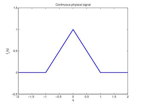
Let us consider \(f_c\) defined by $$\begin{aligned} f_c (\eta) & = \text{tri} (\eta)\\ & = \max \left( 1 - | \eta |, 0 \right) \end{aligned}$$ and can be plotted as follows:
eta=linspace(-2,2,1001);
fc=max(1-abs(eta),0);
plot(eta,fc);
axis([-2 2 -0.5 1.5]);
title('Continuous physical signal');
xlabel('\eta');
ylabel('f_c(\eta)');
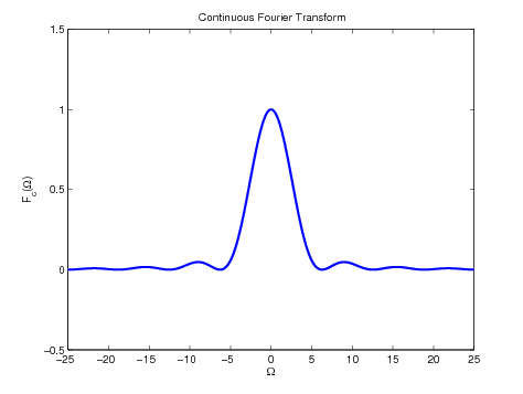
In this case, \(F_c\) can be found analytically and is given by $$\begin{aligned} F_c (\Omega) & = \text{sinc}^2 (\Omega)\\ & = \left( \frac{\sin \left( \frac{\Omega}{2 \pi} \right)}{\frac{\Omega}{2 \pi}} \right)^2 \end{aligned}$$ and can be plotted as follows:
OMEGA=linspace(-25,25,1000);
Fc=(sinc(OMEGA/(2*pi))).^2;
plot(OMEGA,Fc);
axis([-25 25 -0.5 1.5]);
title('Continuous Fourier Transform');
xlabel('Omega');
ylabel('F_c(Omega)');