Section VII

A Hitchhiker's Guide to the FFT

VII. Coming back to the physical space

Fourier transforms are generally used as a tool in order to solve a mathematical problem. Often, one needs to visualise the solution of this problem in the physical space. This is why we need the inverse Fourier transform.

VII.1 Discrete Spectral Inverse Fourier Transform

Let us consider a vector $F_v$, referred to as the discrete spectral function and defined by $$\begin{aligned} F_v : \mathbb{N} & \longrightarrow \mathbb{C}\\ k & \longrightarrow F_v [k] \end{aligned}$$ The Discrete Spectral Inverse Fourier Transform (DSIFT) of $F_v$, denoted $f^{\text{DSIFT}}$ is defined by $$\begin{equation}\begin{aligned} f^{\text{DSIFT}} (\tau) & = \sum_{k = - \infty}^{\infty} F_v [k] e^{j \tau k} \end{aligned}\end{equation}\label{eq:DSIFT}$$ Note that the only differences between equations (\ref{eq:DSIFT}) and II.1.(1) are the names of the variables and the sign in the exponential. Naturally, the DSIFT is continuous in time and $2 \pi$-periodic.

VII.2 Discrete Inverse Fourier Transform

For a given discrete spectral function $F_v$, the $M$-Discrete Inverse Fourier Transform ($M$-DIFT) of $F_v$, denoted $f^{M \text{-} \text{DIFT}}$ is defined in a similar way as in Section III.1 by $$\begin{equation}\begin{aligned} f^{M \text{-} \text{DIFT}} : \left\{ 0, \ldots, M - 1 \right\} & \longrightarrow \mathbb{C} \\ m & \longrightarrow \frac{1}{M} f^{\text{DSIFT}} \left( \frac{2 \pi m}{M} \right) \end{aligned}\end{equation} \label{eq:MDIFT}$$

VII.3 What ifft actually does

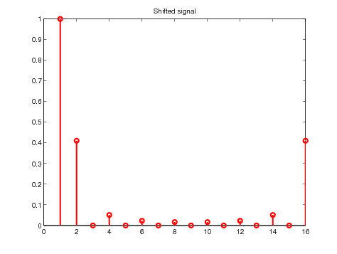
Without surprise, for a given vector X of size M, the Matlab command ifft(X) returns the M-DIFT of X. Again, as for the fft, the spectral signal needs to be ''prepared'' before taking the ifft.

CFT_approx_shift=circshift(CFT_approx,[0 -floor(P/2)]);
stem(CFT_approx_shift,'r');
title('Shifted signal');

Figure 14. Illustration of the signal preparation before taking the ifft

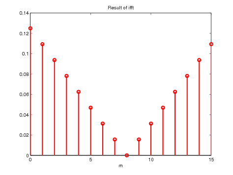
Then we should take the ifft as follows

M=P;
m=0:M-1;
f_ifft=ifft(CFT_approx_shift);
stem(m,real(f_ifft),'r','Linewidth',2);
xlabel('m');
title('Result of ifft');

Figure 15. Output of the ifft function for $M = P$

Again, in order for it to really approximate the original physical function, one needs to make a few modifications to the ifft.

VII.4 Adaptation of the physical axis

First of all, according to Section VII.2, the physical axis must be scaled to pass from $m$ to $\tau$. This can be done by typing

tau_ifft=2*pi*m/M;

The $\eta$-axis of the original function $f_c$ defined in Section I.2 was centred. The physical axis can be centred by typing:

tau_ifft_centred=unwrap(fftshift(tau_ifft)-2*pi);

Finally, in order to pass from $\tau$ to $\eta$ one needs to define the spectral sampling interval $T_s$ and to scale the axis again by typing:

Ts=OMEGA_fft(2)-OMEGA_fft(1);
eta_ifft=1/Ts*tau_ifft_centred;

VII.5 Adaptation of the result vector

In order for the output vector f_ifft to look more like the original function, it needs to be centred. This can be done by typing

f_ifft_centred=fftshift(f_ifft);

It then needs to be scaled according to (\ref{eq:MDIFT}), this can be done by typing

Ts=OMEGA_fft(2)-OMEGA_fft(1);
eta_ifft=1/Ts*tau_ifft_centred;

VII.6 Adaptation of the result vector

In order for the output vector f_ifft to look more like the original function, it needs to be centred. This can be done by typing

f_ifft_centred=fftshift(f_ifft);

It then needs to be scaled according to (\ref{eq:MDIFT}), this can be done by typing

Physical_function_approx=M*Ts/(2*pi)*f_ifft_centred;

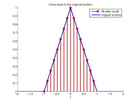
Finally, the plot can be obtained by typing

stem(eta_ifft,real(Physical_function_approx),'r');
hold on
plot(eta,fc,'b');
hold off
legend('ifft after modif','original function');
xlabel('eta');
title('Come back to the original function');

Figure 15. Comparison between the ''adapted'' result of the ifft and the original function