A Hitchhiker's Guide to the FFT
II. Discrete Time Fourier Transform
II.1 Definitions
Given a vector \(f_v\), referred to as the discrete physical function, or sampled physical function and defined by: $$\begin{aligned} f_v : \mathbb{N} & \longrightarrow \mathbb{C}\\ n & \longrightarrow f_v [n], \end{aligned}$$ the Discrete Time Fourier Transform (DTFT) of \(f_v\), denoted \(F^{\text{DTFT}}\), is given by $$\begin{equation}\begin{aligned} F^{\text{DTFT}} (\omega) & = \sum_{n = - \infty}^{\infty} f_v [n] e^{- j \omega n} \label{eq:DTFT} \end{aligned}\end{equation}$$ The vector \(f_v\) is also related to \(F^{\text{DTFT}}\) via Inverse Discrete Time Fourier Transform: $$\begin{equation}\begin{aligned} f_v [n] & = \frac{1}{2 \pi} \int_{- \pi}^{\pi} F^{\text{DTFT}} (\omega) e^{j \omega n} \mathrm{d} \omega . \label{eq:IDTFT} \end{aligned}\end{equation}$$ Note that \(F^{\text{DTFT}}\) is a continuous, \(2 \pi\)-periodic function from \(\mathbb{R} \rightarrow \mathbb{C}\)
II.2 Example
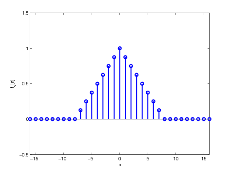
Let us consider the vector \(f_v\) defined by $$\begin{aligned} f_v [n] & = \max (1 - | \eta (n) |, 0), \end{aligned}$$ where $$\begin{aligned} \eta (n) & = 2 n / N \end{aligned}$$ This can be implemented as follows:
N=16;
n=-N:N;
tt=2*n/N;
fvsampled=max(1-abs(tt),0);
stem(n,fvsampled,'b');
xlabel('n');
ylabel('f_v[n]');
axis([-N N -0.5 1.5]);

Figure 3. The vector \(f_v\) for \(N = 16\)
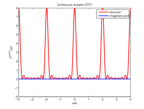
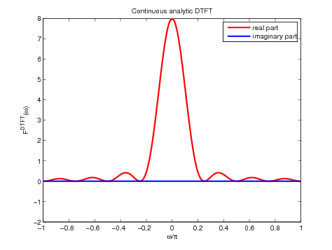
In this case, the DTFT can be computed easily and is given by $$\begin{aligned} F^{\text{DTFT}} (\omega) & = \sum_{n = - \infty}^{\infty} f_v [n] e^{- j \omega n}\\ & = \sum_{n = - N / 2}^{N / 2} (1 - 2| n| / N) e^{- j \omega n} \end{aligned}$$ This can be implemented as follows:
Per=1; % Number of periods one wants to plot
omega=linspace(-Per*pi,Per*pi,1000);
X=zeros(1,numel(omega));
for ii=-N/2:N/2
X=X+fvsampled(ii+N+1)*exp(-1i*omega*(ii));
end
omega_plot=omega/pi;
plot(omega_plot,real(X),'r',omega_plot,imag(X),'b');
title('Continuous analytic DTFT');
axis([-Per Per -2 N/2]); legend('real part','imaginary part');
xlabel('omega/pi'); ylabel('F^{DTFT}(omega)');


Figure 4. Plot of 4 periods (left) and one period (right) of the analytic
DTFT of \(f_v\) for \(N=16\)
